import matplotlib.pyplot as plt
import numpy as np日常工作中经常要用到 matplotlib 来绘图,每次绘图碰到一些细节问题都得谷歌,下次遇到继续谷歌 :) 不知道你是否跟我一样。一方面是自己太懒了,没总结;另一方面,是 matplotlib 实现同一个目标的方式太多了。
比如设置图片标题,可以使用 plt.title(),也可以使用 ax.set_title()。出现这种情况的原因是 matplotlib 提供了两套接口来实现相同的功能:一套是类 MATLAB 工作风格的接口(方便 MATLAB 党丝滑迁移过来),一套是面向对象风格的接口(面向程序员)。这就造成了很多 matplotlib 初学者两种风格代码混用的情况,比如我 :)
这篇文章的主要内容如下:
- 介绍 matplotlib 绘图的基本原理和标准步骤
- 对 MATLAB 风格与面向对象风格做一个比较
- 绘图细节与如何画出精美的图
- 总结数据分析中常用图表的绘图模板代码
matplotlib 是如何绘图的?
matplotlib 内部封装了三层 API:
FigureCanvas:绘图区域;Renderer:可以理解为画笔,控制绘图行为;Artist:如何使用Renderer绘图。
FigureCanvas 和 Renderer 解决与计算机底层的交互问题,Artist 控制点、线、文字、图片等图像要素在绘图区域上展现的细节问题。因此,我们要画出心仪的图像,只需要用好 Artist 对象就可以了 —— 做一个优秀的艺术家!
Artist 对象有两种类型:
- 基础对象(primitives):包括点、线、文字、图片等等我们希望呈现的要素;
- 容器对象(containers):包括画布、坐标轴、坐标系。
不难理解,容器对象是用来放置基础对象的。我们在数学作图的时候,也是先画一个框,再画一个坐标系,坐标轴标好刻度,再作图。与之类似,使用 matplotlib 绘图的标准步骤是:
- 创建一个
figure实例; - 使用
figure实例创建一个或多个Axes或者Subplot实例; - 使用
Axes实例方法创建 primitives。
下面我们就按照这个逻辑来作图。首先我们使用 plt.figure 创建 figure 实例,然后使用 figure.add_axes() 方法创建坐标系,最后使用 plot 方法在坐标系上画图。
NOTE:
figure.add_axes()允许我们在画布任意位置创建坐标系,传入rect=[left, bottom, width, height]参数控制坐标系在画布中位置的百分比。
left, bottom, width, height = (
    0.1,
    0.1,
    0.8,
    0.8,
)  # Quantities are in fractions of figure width and height.
rect = left, bottom, width, height  # the dimension of `Axes` object
fig = plt.figure(
    figsize=(16, 8), dpi=100
)  # create a `figure` object, `figsize` sets the dimension, `dpi` sets pixel units.
ax = fig.add_axes(rect)
ax.plot([1, 2, 3, 4])  # plot y using x as index array 0..N-1
plt.show()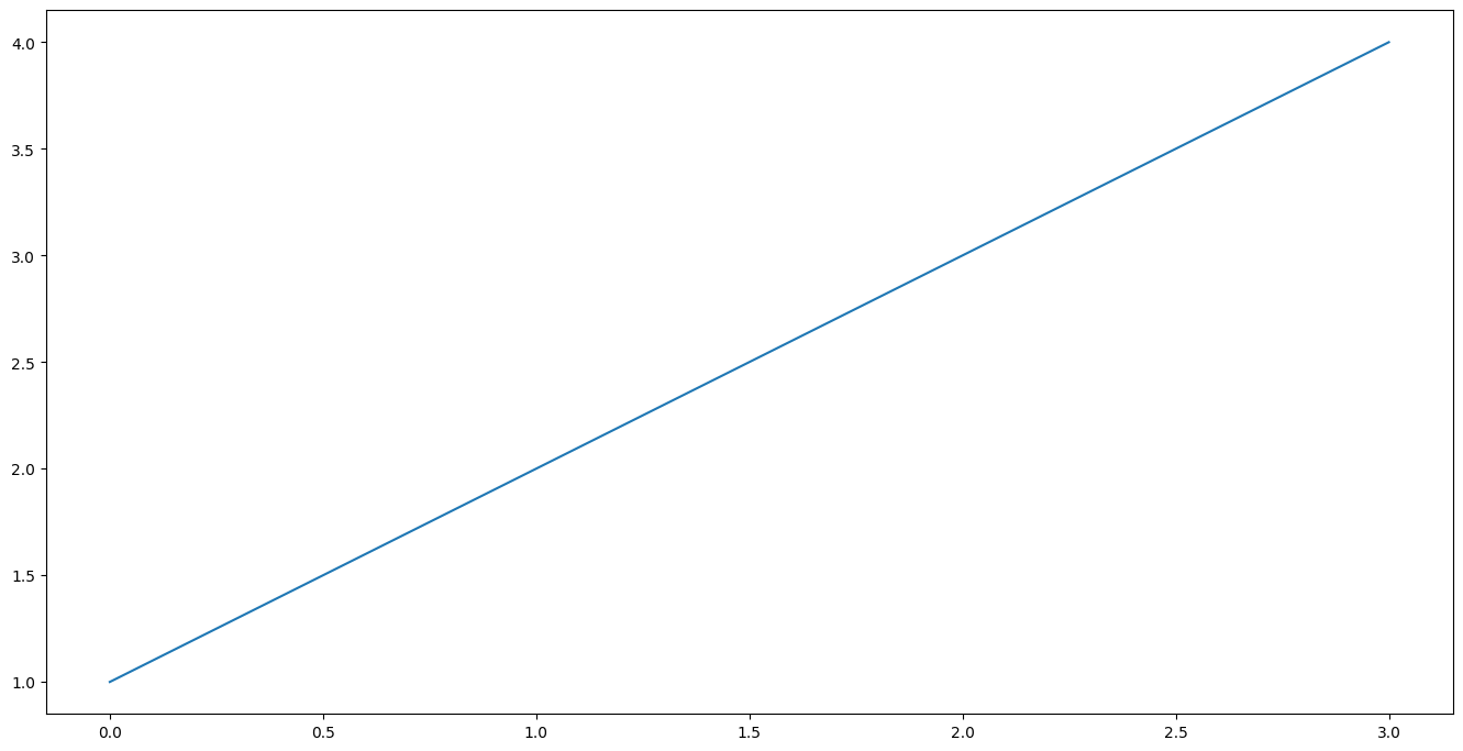
除了添加坐标系,我们还可以使用 figure.add_subplot 方法直接添加子图。子图是 Axes 的一个子类,我们可以把子图看作画布矩阵中的一个元素,每个元素有自己的坐标系,我们可以在上面画图。比如,在下面的代码中,我们创建两个子图。
fig = plt.figure(figsize=(16, 8), dpi=100)
ax1 = fig.add_subplot(2, 1, 1)  # 2 rows, 1 column, the first subplot
ax2 = fig.add_subplot(2, 1, 2)  # 2 rows, 1 column, the second subplot

print("fig.axes: ", fig.axes)
print("ax1.figure:", ax1.figure)
print("ax2.figure: ", ax2.figure)
print("ax1.xaxis: ", ax1.xaxis)
print("ax2.xaxis: ", ax2.xaxis)
print("ax1.yaxis: ", ax1.yaxis)
print("ax2.yaxis: ", ax2.yaxis)
fig.axes: [<Axes: >, <Axes: >]
ax1.figure: Figure(1600x800)
ax2.figure: Figure(1600x800)
ax1.xaxis: XAxis(200.0,424.0)
ax2.xaxis: XAxis(200.0,87.99999999999999)
ax1.yaxis: YAxis(200.0,424.0)
ax2.yaxis: YAxis(200.0,87.99999999999999)
以上输出可以发现,figure 对象包含两个坐标系;ax1 和 ax2 所处的 figure 是一样的;ax1 和 ax2 的坐标轴不一样。
除了先生成图,再添加坐标系,我们也可以使用 plt.subplots() 方法同时生成图和坐标系。比如,下面我们同时生成横向的两个子图,并让它们共享 Y 轴。
# create some toy data
x = [1, 2, 3, 4]
y1 = [1, 2, 3, 4]
y2 = [2, 5, 9, 14]
fig, (ax1, ax2) = plt.subplots(1, 2, sharey=True, figsize=(16, 8), dpi=100)
ax1.plot(x, y1)
ax2.plot(x, y2)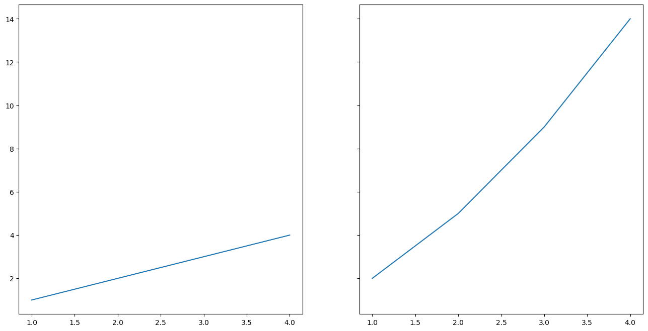
OO-style vs Pyplot-style
在上面的代码中,我们使用了面向对象的风格来使用 matplotlib,即首先显示地创建了图和坐标系实例,再调用它们的方法实现绘图。除此之外,matplotlib 还提供了另一套模仿 MATLAB 的接口,即 Pyplot-style interface。比如下面的代码:
plt.figure(figsize=(16, 8), dpi=100)

plt.plot([1, 2, 3, 4])
plt.title("Pyplot-style")
plt.show()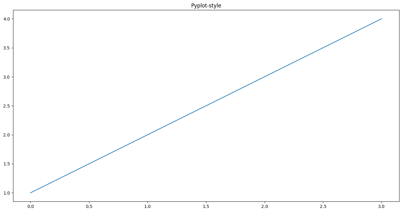
Pyplot-style 接口是基于状态的接口(state-based interface)。我的理解是每调用一次 pyplot 中的命令就会改变一下当前的状态(也就是图像),并将改变之后的状态保存下来,plt.show() 展示最终的状态。而 OO-style 是每次新建一个对象,调用该对象的方法从而在画布上创建新的内容。
两者相比,Pyplot-style 接口简洁,方便我们快速的生成各类图像,但是功能不够强大。OO-style 是官方文档推荐我们使用的方式,功能更加强大,我们可以更自由的控制画布中的元素,从而实现图形的定制。因此,在接下来的内容里,我们都使用 OO-style 的方式来绘图。
画一张精美的图
要画一张精美的图,就需要对 Artist 对象进行定制。首先附上官方文档里的这张图。

我们可以对各种 Aritst 类型对象进行定制,包括:
- 画布
- 坐标系
- 坐标轴
- 点、线
- 文字
- 图例
- annotation
坐标轴
matplotlib 的 Axes 是绘图的入口。一旦在图上放置了一个 Axes,就可以使用许多方法向Axes 添加数据。一个 Axes 通常具有一对 Axis Artists,它们定义了数据坐标系,并包括添加注释(如 x 轴和 y 轴标签、标题和图例)的方法。
fig, ax = plt.subplots(figsize=(16, 8), layout="constrained")
np.random.seed(19680801)
t = np.arange(200)
x = np.cumsum(np.random.randn(200))
y = np.cumsum(np.random.randn(200))

linesx = ax.plot(t, x, label="Random walk x")
linesy = ax.plot(t, y, label="Random walk y")

# 设置 x 轴标签
ax.set_xlabel("Time [s]")
# 设置 y 轴标签
ax.set_ylabel("Distance [km]")
# 设置标题
ax.set_title("Random walk example")
ax.legend()
plt.show()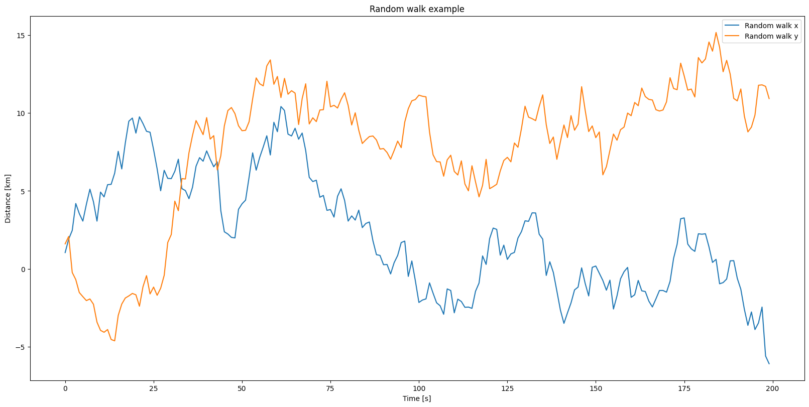
也可以使用 set_xlim 和 set_ylim 方法设置坐标轴的范围,可以使用 set_xscale 和 set_yscale 设置坐标轴的比例尺度。
fig, ax = plt.subplots(figsize=(16, 8), layout="constrained")
np.random.seed(19680801)
t = np.arange(200)
x = 2 ** np.cumsum(np.random.randn(200))
linesx = ax.plot(t, x)
ax.set_yscale("log")
ax.set_xlim([20, 180])
plt.show()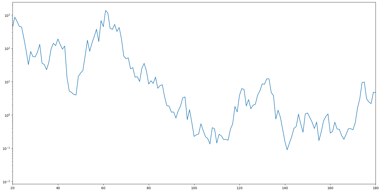
Axes 类还提供了处理坐标轴刻度及其标签的辅助方法。其中最直接的是 set_xticks 和 set_yticks,它们可以手动设置刻度的位置,以及可选地设置它们的标签。可以使用minorticks_on 或 minorticks_off 来切换次要刻度。
fig, ax = plt.subplots(figsize=(16, 8), layout="constrained")

xx = np.arange(0, 2 * np.pi, 0.01)
ax.plot(xx, np.sin(xx))

ax2 = ax.twinx()

# 设置刻度和标签
ax2.set_yticks(
    [0.0, 0.5 * np.pi, np.pi, 1.5 * np.pi, 2 * np.pi],
    labels=["$0$", r"$\frac{1}{2}\pi$", r"$\pi$", r"$\frac{3}{2}\pi$", r"$2\pi$"],
)
# 开启次要刻度
plt.minorticks_on()
plt.show()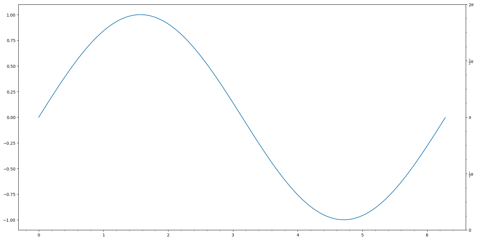
也可以使用 tick_params 调整 Axes 刻度和刻度标签:
fig, ax = plt.subplots(figsize=(16, 8))
ax.plot(np.arange(10))
ax.tick_params(top=True, labeltop=True, color="red", axis="x", labelcolor="green")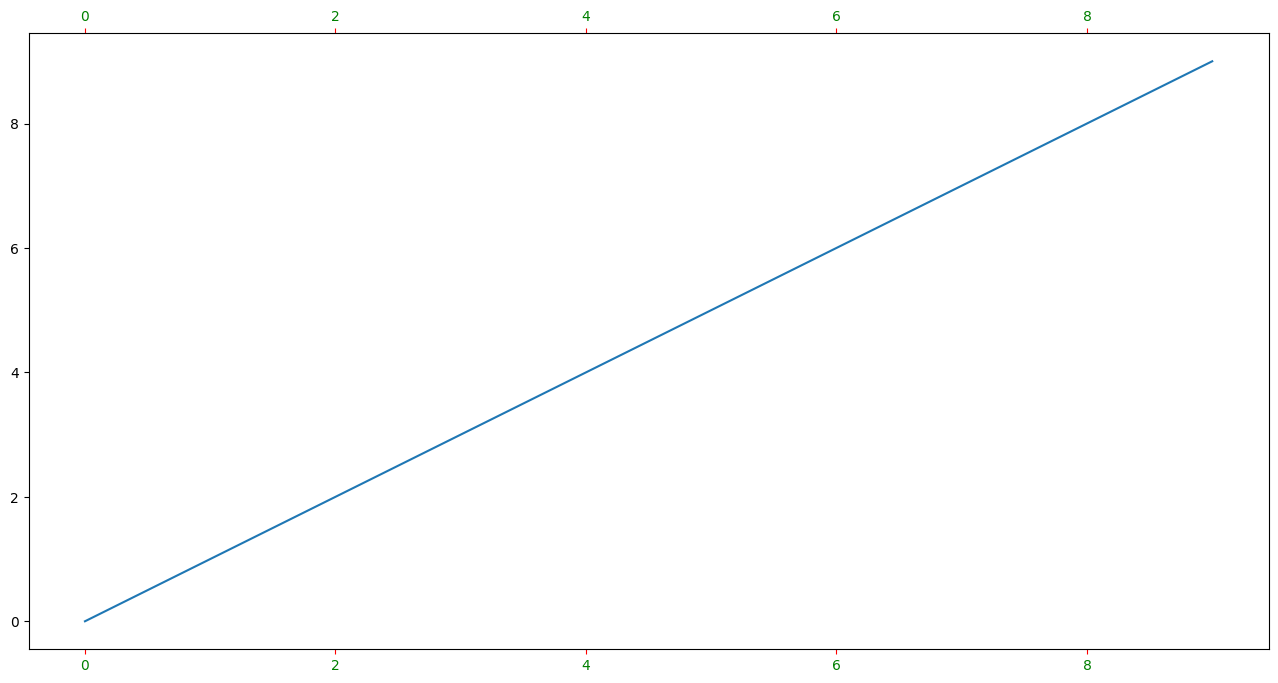
线
matplotlib 中的线是一个 line2D 对象,它有很多属性,我们可以通过对属性进行修改实现对线的美化和定制。这里,列出一些比较常用的属性:
color或者c:线的颜色;alpha:透明度;linewidth:线的宽度;linestyle或者ls;-或者solid:实线;--或者dashed:短划线;-.或者dashdot:点划线;:或者dotted:点虚线;
marker或则m:.:点o:圆圈^:上三角形+:加号x:Xs:正方形*:五角星
下面,我们在代码中来看一下各种属性的使用:
# create some toy data
data1, data2, data3, data4 = np.random.randn(4, 100)

fig, ax = plt.subplots(figsize=(16, 8), dpi=100)

ax.plot(
    np.cumsum(data1), color="black", linewidth="3", linestyle="-", marker="o", alpha=0.5
)
ax.plot(np.cumsum(data2), color="red", linestyle="--", marker="^")
ax.plot(np.cumsum(data3), color="green", linestyle="-.", marker="+")
ax.plot(np.cumsum(data4), color="orange", linestyle=":", marker="x")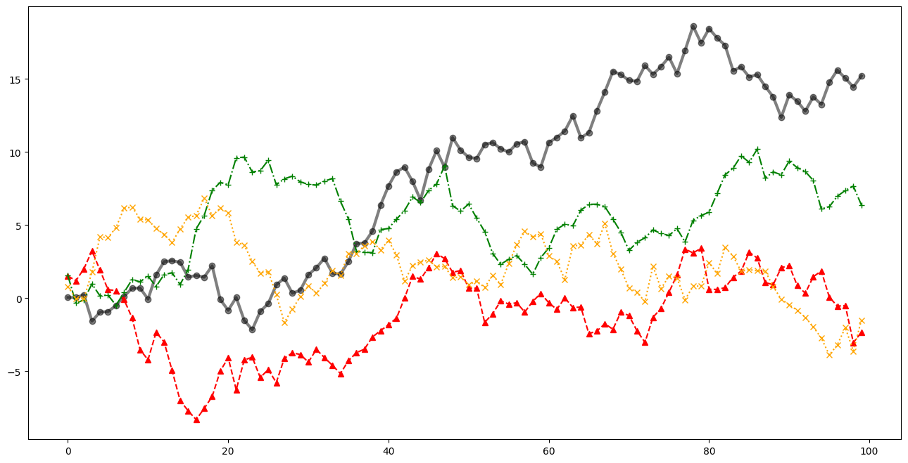
我们也可以使用对应的方法来设置或者修改属性值。ax.plot() 方法返回一个 line2D 对象列表,我们可以在对应的 line2D 对象上调用方法。比如,我们可以使用 set_linestyle() 方法修改 linestyle 属性,可以使用 set_marker() 方法修改 marker 属性。
fig, ax = plt.subplots(figsize=(16, 8), dpi=100)

(l,) = ax.plot(np.cumsum(data1))
l.set_linestyle("--")
l.set_marker("x")
data1, data2, data3, data4 = np.random.randn(4, 100)fig, ax = plt.subplots(figsize=(16, 8))
x = np.arange(len(data1))
ax.plot(x, np.cumsum(data1), color="blue", linewidth=3, linestyle="--")
l = ax.plot(x, np.cumsum(data2), color="orange", linewidth=2, linestyle=":")
# l.set_linestyle(':')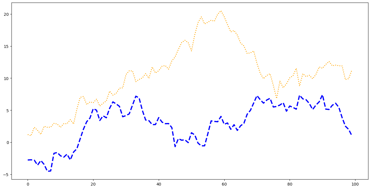
文字
matplotlib 中的文字是一个 matplotlib.text.Text 对象,利用相关的属性我们可以控制文字显示的样式,包括文字位置、显示的字体、字体大小、颜色等等。
alpha:透明度fontfamily:FONTNAME, ‘serif’, ‘sans-serif’, ‘cursive’, ‘fantasy’, ‘monospace’fontsize:float or ‘xx-small’, ‘x-small’, ‘small’, ‘medium’, ‘large’, ‘x-large’, ‘xx-large’fontweight:a numeric value in range 0-1000, ‘ultralight’, ‘light’, ‘normal’, ‘regular’, ‘book’, ‘medium’, ‘roman’, ‘semibold’, ‘demibold’, ‘demi’, ‘bold’, ‘heavy’, ‘extra bold’, ‘black’fontstyle:‘normal’, ‘italic’, ‘oblique’
这里放上官方文档的例子:
fig = plt.figure(figsize=(16, 8))
ax = fig.add_subplot()
fig.subplots_adjust(top=0.85)

# Set titles for the figure and the subplot respectively
fig.suptitle("bold figure suptitle", fontsize=14, fontweight="bold")
ax.set_title("axes title")

ax.set_xlabel("xlabel")
ax.set_ylabel("ylabel")

# Set both x- and y-axis limits to [0, 10] instead of default [0, 1]
ax.axis([0, 10, 0, 10])

ax.text(
    3,
    8,
    "boxed italics text in data coords",
    style="italic",
    bbox={"facecolor": "red", "alpha": 0.5, "pad": 10},
)

ax.text(2, 6, r"an equation: $E=mc^2$", fontsize=15)

ax.text(3, 2, "Unicode: Institut für Festkörperphysik")

ax.text(
    0.95,
    0.01,
    "colored text in axes coords",
    verticalalignment="bottom",
    horizontalalignment="right",
    transform=ax.transAxes,
    color="green",
    fontsize=15,
)

ax.plot([2], [1], "o")
ax.annotate(
    "annotate",
    xy=(2, 1),
    xytext=(3, 4),
    arrowprops=dict(facecolor="black", shrink=0.05),
)

plt.show()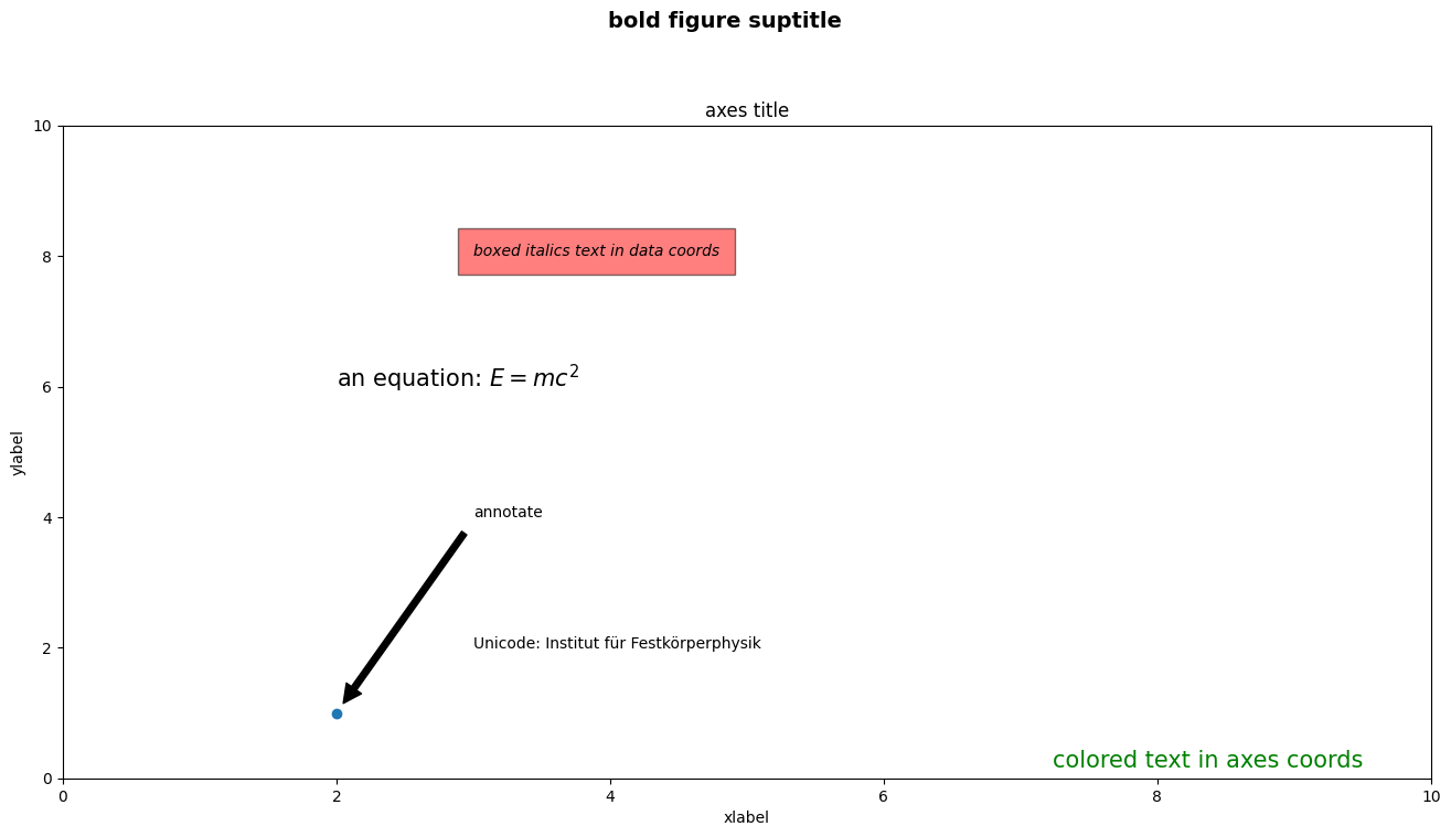
图例
data1, data2, data3, data4 = np.random.randn(4, 100)

fig, ax = plt.subplots(figsize=(16, 8), dpi=100)

ax.plot(
    np.cumsum(data1),
    color="black",
    linewidth="3",
    linestyle="-",
    marker="o",
    label="data1",
)
ax.plot(np.cumsum(data2), color="red", linestyle="--", marker="^", label="data2")
ax.plot(np.cumsum(data3), color="green", linestyle="-.", marker="+", label="data3")
ax.plot(np.cumsum(data4), color="orange", linestyle=":", marker="x", label="data4")

ax.legend(loc="best", frameon=False)
plt.show()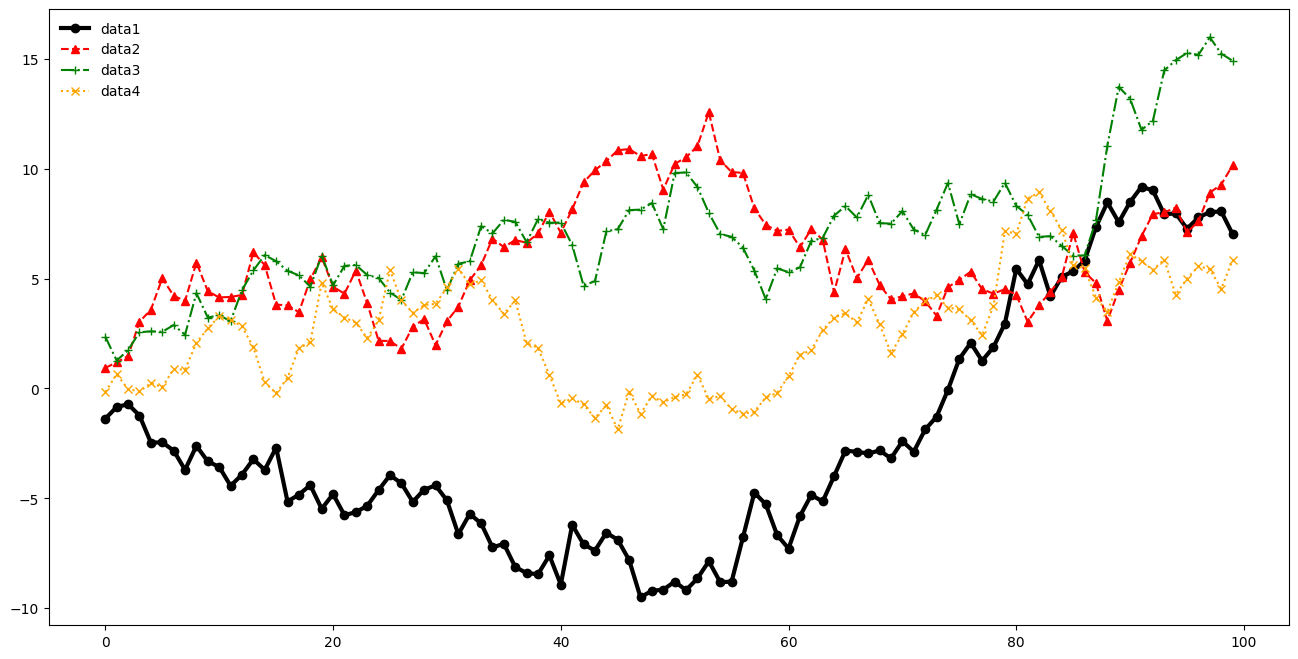
Spines
data1, data2, data3, data4 = np.random.randn(4, 100)

fig, ax = plt.subplots(figsize=(16, 8), dpi=100)

ax.plot(
    np.cumsum(data1),
    color="black",
    linewidth="3",
    linestyle="-",
    marker="o",
    label="data1",
)
ax.plot(np.cumsum(data2), color="red", linestyle="--", marker="^", label="data2")
ax.plot(np.cumsum(data3), color="green", linestyle="-.", marker="+", label="data3")
ax.plot(np.cumsum(data4), color="orange", linestyle=":", marker="x", label="data4")

ax.legend(loc="best", frameon=False)

# Remove the plot frame lines. They are unnecessary chartjunk.
ax.spines["top"].set_visible(False)
ax.spines["right"].set_visible(False)

plt.show()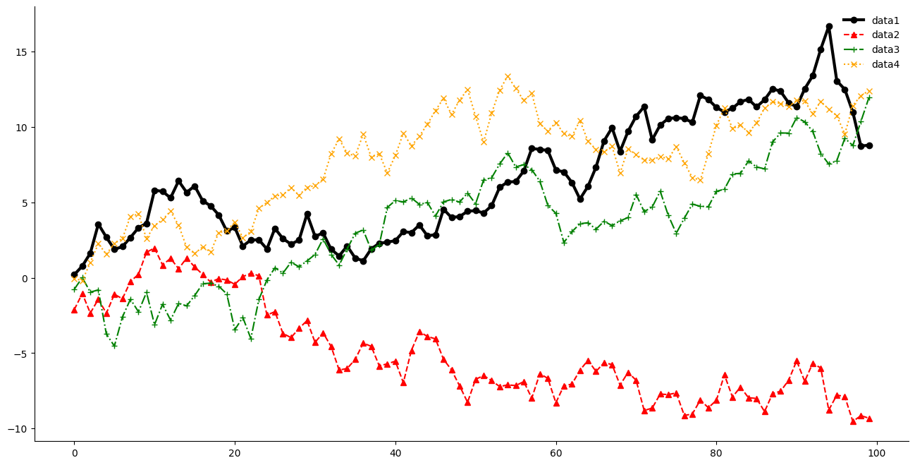
References
- https://matplotlib.org/matplotblog/posts/pyplot-vs-object-oriented-interface/
- https://stackoverflow.com/questions/52816131/matplotlib-pyplot-documentation-says-it-is-state-based-interface-to-matplotlib
- https://matplotlib.org/stable/tutorials/introductory/usage.html#styling-artists