因为经常要计算 CAR，所以写了一个脚本，支持市场模型和三因子模型，测试数据都来自于国泰安数据库，视频介绍在 b 站。

脚本的核心是 EventStudy 类。下面是一个简单的例子：

import eventstudy

es_market_model = eventstudy.EventStudy(
    sample_market_model,  # 事件样本
    "Market",  # 正常收益率估计模型
    market_model_data, # 估计模型所需数据
    daily_stock_returns,  # 个股历史回报率
    -1,  # t1
    30,  # t2
    10,  # span
    200  # 估计期长度
)

市场模型

R_{it} = \alpha_i + \beta_iR_{Mt} + \varepsilon_{it}

R_{it} 表示公司 i 在第 t 个交易日的考虑现金红利再投资的个股回报率，R_{Mt} 表示第 t 个交易日公司所在分市场的市场回报率，等于考虑现金红利再投资的日市场回报率（流通市值加权平均法）。

import pandas as pd
import eventstudy

daily_stock_returns = pd.read_csv(
    "./data/daily_stocks_returns.csv", dtype={"ticker": str}
)

daily_stock_returns 是个股历史回报率，注意个股历史回报率需要包含如下测试字段，即 ticker、TradingDate 和 return，分别代表股票代码、交易日和个股回报率。

daily_stock_returns.head()

	ticker	TradingDate	return
0	000001	2013-11-29	-0.001468
1	000001	2013-12-02	0.011029
2	000001	2013-12-03	-0.015273
3	000001	2013-12-04	0.004431
4	000001	2013-12-05	-0.012500

sample_market_model = pd.read_csv(
    "./data/sample_for_marketmodel.csv", dtype={"ticker": str}
)

sample_market_model 是事件样本，注意事件样本需要包含如下测试字段，即 EventDate、ticker 和 MarketTypeID，分别代表事件日、股票代码和市场类型。

sample_market_model.head()

	EventDate	ticker	MarketTypeID
0	2016-04-21	002177	4
1	2016-11-10	300188	16
2	2018-01-12	300002	16
3	2018-01-15	000935	4
4	2018-01-15	000021	4

market_model_data 是市场模型所需要的数据，注意市场模型数据需要包含如下测试字段，即 MarketTypeID、TradingDate 和 market_returns，分别代表市场类型、交易日和市场收益率。

market_model_data = pd.read_csv("./data/market_model_data.csv")

market_model_data.head()

	MarketTypeID	TradingDate	market_returns
0	1	1990-12-19	NaN
1	1	1990-12-20	0.050067
2	1	1990-12-21	0.039671
3	1	1990-12-24	0.049380
4	1	1990-12-25	0.049938

es_market_model = eventstudy.EventStudy(
    sample_market_model.head(10),
    "Market",
    market_model_data,
    daily_stock_returns,
    -1,
    30,
    10,
    200,
)

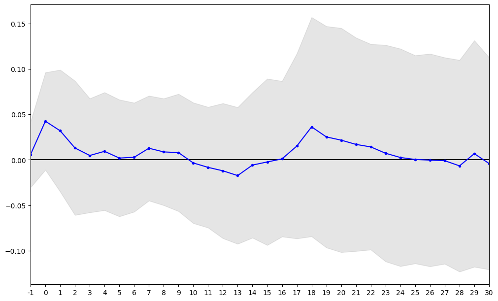
res_market_model = es_market_model.get_result()

Tasks finished: 100%

get_result() 返回一个字典，字典中包含样本 CAR、CAR 的描述性统计结果、剔除的样本和剩余样本。

res_market_model.keys()

dict_keys(['describe_res', 'sample_removed', 'sample_remained', 'sample_cars'])

res_market_model["sample_remained"]

	EventDate	ticker	MarketTypeID
0	2016-04-21	002177	4
1	2016-11-10	300188	16
2	2018-01-12	300002	16
3	2018-01-15	000935	4
4	2018-01-15	000021	4
5	2018-01-30	300108	16
6	2018-04-05	600602	1
7	2018-12-11	300356	16
8	2019-05-08	300427	16
9	2019-07-02	000917	4

eventstudy.res_plot(re_market_model["sample_cars"], 0.90)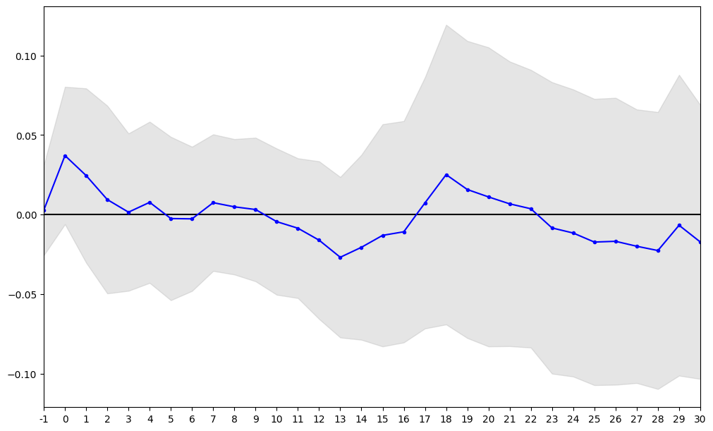

三因子模型

R_{it} - R_{ft} = \alpha_i + b_i(R_{Mt}-R_{ft}) + s_iSMB_t + h_iHML_t + \varepsilon_it

famafrench_factors = pd.read_csv("./data/famafrench_factors_data.csv")

famafrench_factors 是三因子模型数据，注意三因子数据需要包含如下测试字段，即 MarketTypeID、TradingDate、RiskPremium、SMB、HML 和 risk_free_rate，分别代表市场类型、交易日、风险溢价因子、SMB、HML 和无风险利率。

famafrench_factors.head()

	MarketTypeID	TradingDate	RiskPremium	SMB	HML	risk_free_rate
0	P9706	1990-12-19	2.473374	NaN	NaN	0.0227
1	P9710	1990-12-19	2.473374	NaN	NaN	0.0227
2	P9709	1990-12-19	2.473374	NaN	NaN	0.0227
3	P9712	1990-12-19	2.473374	NaN	NaN	0.0227
4	P9713	1990-12-19	2.473374	NaN	NaN	0.0227

sample_famafrench = pd.read_csv("./data/sample.csv", dtype={"ticker": str})

sample_famafrench 是事件样本，与前述要求一致，需要包含如下测试字段。

sample_famafrench.head()

	EventDate	ticker	MarketTypeID
0	2016-04-21	002177	P9706
1	2016-11-10	300188	P9705
2	2018-01-12	300002	P9705
3	2018-01-15	000935	P9706
4	2018-01-15	000021	P9706

es_famafrench = eventstudy.EventStudy(
    sample_famafrench.head(10),
    "FamaFrench",
    famafrench_factors,
    daily_stock_returns,
    -1,
    30,
    10,
    200,
)

res_famafrench = es_famafrench.get_result()

Tasks finished: 100%

res_famafrench.keys()

dict_keys(['describe_res', 'sample_removed', 'sample_remained', 'sample_cars'])

res_famafrench["describe_res"]

	count	mean	std	min	25%	50%	75%	max	t-statstics	p-value
-1	10.0	0.005946	0.050654	-0.042915	-0.026691	-0.008127	0.004223	0.102982	0.371196	0.719079
0	10.0	0.042546	0.074948	-0.035565	-0.010073	0.022935	0.060273	0.202987	1.795155	0.106202
1	10.0	0.031981	0.093752	-0.069651	-0.007391	-0.003999	0.021624	0.263352	1.078718	0.308774
2	10.0	0.013060	0.103207	-0.101936	-0.029064	-0.023455	0.024744	0.232986	0.400162	0.698369
3	10.0	0.004802	0.087637	-0.130160	-0.043901	-0.016113	0.064789	0.143388	0.173265	0.866277
4	10.0	0.009385	0.090681	-0.128522	-0.046949	-0.022871	0.092813	0.147597	0.327286	0.750935
5	10.0	0.001967	0.089825	-0.153967	-0.036466	-0.013752	0.072597	0.134979	0.069254	0.946301
6	10.0	0.002818	0.083841	-0.180795	-0.027049	0.003889	0.059211	0.121202	0.106300	0.917676
7	10.0	0.012787	0.080665	-0.159540	-0.014551	0.020998	0.050448	0.150747	0.501306	0.628188
8	10.0	0.008737	0.082093	-0.163451	-0.025143	0.023856	0.041238	0.142756	0.336549	0.744171
9	10.0	0.007964	0.090177	-0.153678	-0.022929	0.023700	0.070196	0.139917	0.279291	0.786334
10	10.0	-0.003413	0.092743	-0.155530	-0.031332	0.009525	0.043308	0.138305	-0.116377	0.909909
11	10.0	-0.008281	0.092809	-0.184369	-0.031162	0.005624	0.017887	0.132797	-0.282173	0.784192
12	10.0	-0.012063	0.103813	-0.200354	-0.033344	0.006032	0.039354	0.143062	-0.367457	0.721771
13	10.0	-0.017322	0.105090	-0.222945	-0.021649	-0.004715	0.024077	0.145804	-0.521229	0.614789
14	10.0	-0.005754	0.111856	-0.203818	-0.031657	-0.013775	0.070799	0.152910	-0.162683	0.874362
15	10.0	-0.002302	0.127973	-0.219148	-0.050842	-0.027914	0.074407	0.224666	-0.056889	0.955877
16	10.0	0.001072	0.119628	-0.205463	-0.060483	-0.022024	0.098753	0.177393	0.028340	0.978010
17	10.0	0.015176	0.142262	-0.169627	-0.069435	-0.026533	0.128153	0.254051	0.337348	0.743589
18	10.0	0.036296	0.168552	-0.138709	-0.067674	-0.031261	0.149025	0.306288	0.680958	0.513035
19	10.0	0.025216	0.170236	-0.203934	-0.074913	-0.028633	0.146160	0.305098	0.468413	0.650627
20	10.0	0.021668	0.172407	-0.194432	-0.079519	-0.053014	0.160581	0.333420	0.397440	0.700304
21	10.0	0.016986	0.164136	-0.170316	-0.096441	-0.043403	0.144772	0.317196	0.327251	0.750961
22	10.0	0.014237	0.158083	-0.164113	-0.086671	-0.046541	0.129103	0.284242	0.284792	0.782248
23	10.0	0.007261	0.166520	-0.155520	-0.115051	-0.052748	0.123317	0.313846	0.137894	0.893360
24	10.0	0.002597	0.167286	-0.163574	-0.109552	-0.051470	0.117628	0.328568	0.049084	0.961924
25	10.0	0.000427	0.160041	-0.160845	-0.106606	-0.054970	0.107540	0.310538	0.008434	0.993455
26	10.0	-0.000277	0.163577	-0.144695	-0.116407	-0.067567	0.126459	0.307726	-0.005351	0.995848
27	10.0	-0.000930	0.158710	-0.126786	-0.114920	-0.073548	0.098323	0.323083	-0.018528	0.985622
28	10.0	-0.006622	0.162787	-0.141247	-0.117763	-0.075430	0.085477	0.329415	-0.128646	0.900467
29	10.0	0.006816	0.174149	-0.130723	-0.116153	-0.079282	0.140219	0.336229	0.123763	0.904223
30	10.0	-0.004030	0.163063	-0.161690	-0.112566	-0.068521	0.070614	0.332546	-0.078147	0.939421

eventstudy.res_plot(res_famafrench["sample_cars"])